Difference Between Linear Regression and Logistic Regression#
Both linear regression and logistic regression study factors that influence a dependent variable, but they apply to different types of dependent variables.
- Linear regression: the dependent variable is continuous, for example scale items can be treated as continuous data. If there are multiple independent variables, it is called multiple linear regression. If there is only one independent variable, it is simple linear regression.
- Logistic regression: the dependent variable is grouped, such as categorical variables like gender or grade. Binary logistic regression is used for binary variables, and multinomial logistic regression is used for multi-category variables.
Steps#
Calculate averages for scale dimensions:
- Transform > Compute Variable
- Enter the dimension name as the target variable, and enter
mean(first item under the dimension to last item under the dimension)as the numeric expression.- For example, you do not need to type the item names manually; just click the corresponding labels on the left:
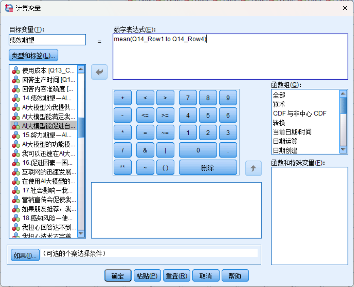
- For example, you do not need to type the item names manually; just click the corresponding labels on the left:
- Perform the same operation for all dimensions.
Choose regression analysis: in the menu bar, click “Analyze” > “Regression” > “Linear.”
Set variables: in the dialog box, drag the dependent variable into the “Dependent” box and the independent variables into the “Independent(s)” box.
Choose statistics: click the “Statistics” button, and select “Collinearity diagnostics” and “Durbin-Watson (U).”
Generate charts: in the “Plots” option, enter
Y:\*ZRESID; X:\*ZPRED, and select Histogram (H) and Normal probability plot (R).
Result Interpretation#
Model Summary#
R-squared: It is the proportion of variance in the dependent variable (predicted variable) explained by the independent variables (predictors). For example, if R-squared = 0.799, the predictors can explain 79.9% of the change in the dependent variable. In general, an R-squared greater than 50% indicates that the model has good explanatory power. Adjusted R-squared: A correction of R-squared that considers the effect of the number of independent variables. R-squared may increase when independent variables are added even if the newly added variables have no predictive ability. Adjusted R-squared penalizes nonsignificant variables, making model-fit evaluation more accurate. Durbin-Watson: also called the D-W value. It is used to detect autocorrelation in model residuals. A value close to 2 indicates no significant autocorrelation among residuals. A value below 2 indicates positive autocorrelation, while a value above 2 indicates negative autocorrelation. For example, a Durbin-Watson value of 1.972 is close to 2, indicating almost no significant autocorrelation among model residuals, so sample independence is basically satisfied.
ANOVA#
When the significance p-value is less than 0.05, at least one independent variable has a significant effect on the dependent variable, meaning the model is statistically significant.
Coefficients#
Significance < 0.05: the independent variable has a significant effect on the dependent variable. If a variable’s significance is greater than 0.05, consider removing that variable and running the regression again.
VIF < 5 (sometimes the standard is < 10): indicates no multicollinearity, and the result is accurate and reliable. If a variable’s VIF exceeds this range, consider removing that variable and retesting.
Regression equation: the final regression equation is: dependent variable = ∑B × independent variable
- B is the unstandardized regression coefficient, plus the constant.
- beta, the standardized regression coefficient, does not include the constant.
Plots#
- Histogram: the ideal distribution has a low-high-low bell shape.
- P-P plot: data points should fall along the diagonal line, indicating consistency between the data and the normal distribution.
Word Explanation#
| R-squared | Adjusted R-squared | Durbin-Watson | P |
|---|---|---|---|
| 0.795 | 0.792 | 2.018 | <0.001 |
a Predictors: (constant), personal innovativeness, facilitating conditions, price value, social influence b Dependent variable: behavioral intention
According to the table, the adjusted R-squared is 0.792, meaning the predictors can explain 79.2% of the variation in behavioral intention. The Durbin-Watson coefficient is 2.018, close to 2, indicating almost no autocorrelation among model residuals; therefore, the data are independent. The model p-value is less than 0.05, meaning the model is significant and the independent variables can explain changes in the dependent variable.
| Dimension | Regression coefficient | Significance | Tolerance | VIF |
|---|---|---|---|---|
| Facilitating conditions | 0.217 | <0.001 | 0.253 | 3.96 |
| Social influence | 0.115 | 0.033 | 0.279 | 3.583 |
| Price value | 0.416 | <0.001 | 0.355 | 2.82 |
| Personal innovativeness | 0.24 | <0.001 | 0.366 | 2.736 |
| a Dependent variable: behavioral intention |
The regression equation is: Behavioral intention = 0.217 * facilitating conditions + 0.115 * social influence + 0.416 * price value + 0.24 * personal innovativeness
The table shows that all independent variables have significance values below 0.05 and all VIF values are below 5, indicating no multicollinearity. The model is valid, and the independent variables can sufficiently explain the dependent variable.