Data Presentation Forms#
When conducting normality tests, data are usually presented in the following two ways:
- Normally distributed data: presented with the mean (M) and standard deviation (SD), suitable for parametric tests such as t tests and ANOVA.
- Non-normally distributed data: presented with the median and interquartile range (IQR), suitable for nonparametric tests.
However, in questionnaire analysis, parametric tests are still used in most cases, and data are presented as mean ± standard deviation (M±SD).
- Independent-samples t test: used to compare a binary grouping variable, such as gender: male/female, with a continuous dependent variable, such as score.
- One-way analysis of variance (ANOVA): used to compare a multi-category variable (factor) with a continuous dependent variable, such as score.
Preliminary Variable Operation#
- Transform > Compute Variable
- Enter the dimension name as the target variable, and enter
mean(first item under the dimension to last item under the dimension)as the numeric expression.
- For example, you do not need to type the item names manually; just click the corresponding labels on the left:
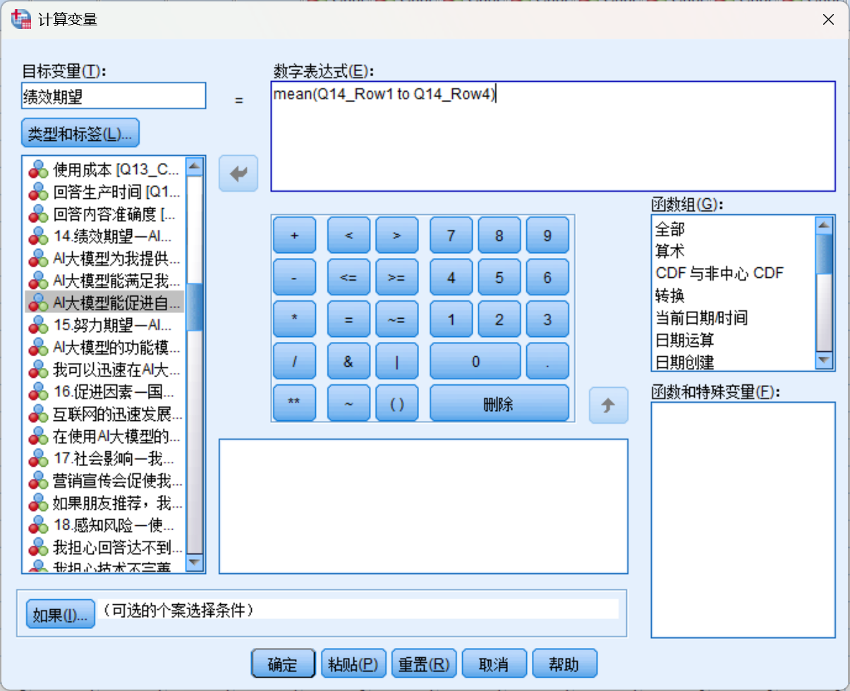
- Perform the same operation for all dimensions.
Independent-Samples t Test#
Operation Steps#
- Choose the analysis method: click “Analyze” > “Compare Means” > “Independent-Samples T Test” in the menu bar.
- Set variables: in the dialog box, add the dependent variable to the “Test Variable(s)” box and add the grouping variable to the “Grouping Variable” box. Click “Define Groups,” enter the values of the grouping variable, such as male = 1 and female = 2, then click “Continue.”
- Choose options: click the “Options” button and select “Mean and standard deviation” and “Significance level” to output relevant statistics and significance-test results.
- Run the analysis: after setting everything, click “OK” to run the analysis.
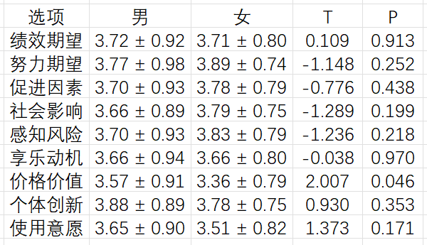
- Draw the table as follows:
Result Interpretation#
Descriptive statistics: check each group’s mean, standard deviation, and sample size. For example, boys’ average score is 80 and girls’ average score is 85.
Homogeneity of variance test: in the “Levene’s Test for Equality of Variances” table, check the “Sig.” value. If the significance value is greater than 0.05, the homogeneity-of-variance assumption holds, so read the “Equal variances assumed” row. If it is less than 0.05, variance is unequal, so read the “Equal variances not assumed” row. For example, Sig. = 0.653 > 0.05, indicating homogeneity of variance.
t-test result: in the “t-test” table, check the “Sig.” value. If the Sig. value is less than 0.05, the difference between the two group means is significant; if it is greater than 0.05, the difference is not significant. For example, Sig. = 0.116 > 0.05, indicating no significant difference.
T: the t value is calculated from the sample data and is used to measure the relationship between the sample mean difference and sample variability.
- A larger t value indicates a larger mean difference between the two groups and relatively smaller variability, suggesting the between-group difference may be more significant.
- A smaller t value indicates a smaller mean difference, which may suggest no significant difference between the two groups.
One-Way Analysis of Variance (ANOVA)#
Operation Steps#
- Choose the analysis method: click “Analyze” > “Compare Means” > “One-Way ANOVA” in the menu bar.
- Set variables: in the dialog box, add the dependent variable to the “Dependent List” box and add the factor to the “Factor” box.
- Choose options: click the “Options” button and select “Descriptive.”
- Run the analysis: after setting everything, click “OK” to run the analysis.
Result Interpretation#
- Descriptive statistics: check each group’s mean, standard deviation, and sample size. For example, teaching method A has an average score of 75, B has 80, and C has 85.
- ANOVA result: in the “ANOVA” table, check the “Sig.” value. If the Sig. value is less than 0.05, the mean difference among groups is significant; if it is greater than 0.05, the difference is not significant. For example, Sig. = 0.116 > 0.05, indicating no significant difference.
- F value: reflects the ratio of between-group differences to within-group differences.
Supplement#
If you want further analysis, run post hoc comparisons for variables with significant differences: Post Hoc — LSD under equal variances assumed.
Interpretation:#
- Mean difference (I - J):
- This value represents the mean difference between two groups. If it is positive, the mean of the first group (I group) is greater than that of the second group (J group). If it is negative, the mean of the first group is lower than that of the second group.
- Significance (Sig.):
- If the p-value is < 0.05, the mean difference between the two groups is significant.
- If the p-value is ≥ 0.05, the difference is not significant.
Result Display:#
- Rows to keep: dependent variable, I, J, I-J, significance
- Columns to keep: groups with p-value < 0.05
Word Explanation#
- Independent-samples t test
| Option | Male | Female | T | P |
|---|---|---|---|---|
| Performance expectancy | 3.72 ± 0.92 | 3.71 ± 0.80 | 0.109 | 0.913 |
| Effort expectancy | 3.77 ± 0.98 | 3.89 ± 0.74 | -1.148 | 0.252 |
| Facilitating conditions | 3.70 ± 0.93 | 3.78 ± 0.79 | -0.776 | 0.438 |
| Social influence | 3.66 ± 0.89 | 3.79 ± 0.75 | -1.289 | 0.199 |
| Perceived risk | 3.70 ± 0.93 | 3.83 ± 0.79 | -1.236 | 0.218 |
| Hedonic motivation | 3.66 ± 0.94 | 3.66 ± 0.80 | -0.038 | 0.970 |
| Price value | 3.57 ± 0.91 | 3.36 ± 0.79 | 2.007 | 0.046 |
| Personal innovativeness | 3.88 ± 0.89 | 3.78 ± 0.75 | 0.930 | 0.353 |
| Behavioral intention | 3.65 ± 0.90 | 3.51 ± 0.82 | 1.373 | 0.171 |
There is no significant difference between men and women on most options. Only the mean difference for “price value” is significant (P = 0.046), indicating a significant gender difference in perceived price value.
This finding shows that gender plays an important role in price sensitivity and value perception. Future research can further explore the reasons behind this difference and analyze possible sociocultural factors or psychological mechanisms. Meanwhile, companies and brands can design more personalized marketing strategies and campaigns for different genders to improve targeting and market competitiveness. For example, men and women may respond differently to price discounts and promotions, so customized pricing strategies may help improve sales outcomes.
- One-way analysis of variance (ANOVA)
| Dimension | Freshman | Sophomore | Junior | Senior | Master’s | Doctoral | F value | P value |
|---|---|---|---|---|---|---|---|---|
| Performance expectancy | 3.79±0.87 | 3.66±0.85 | 3.49±0.82 | 3.62±0.93 | 3.77±0.58 | 4.17±0.88 | 0.873 | 0.5 |
| Effort expectancy | 3.92±0.81 | 3.67±1.00 | 3.56±0.73 | 3.96±0.89 | 4.10±0.42 | 2.89±1.71 | 2.329 | 0.043 |
| Facilitating conditions | 3.90±0.77 | 3.61±0.91 | 3.16±0.84 | 3.65±1.00 | 4.08±0.58 | 4.11±0.77 | 4.28 | 0.001 |
| Social influence | 3.80±0.82 | 3.51±0.89 | 3.41±0.65 | 3.86±0.86 | 4.21±0.50 | 3.67±0.33 | 2.881 | 0.015 |
| Perceived risk | 3.79±0.82 | 3.66±0.94 | 3.48±0.86 | 3.91±0.84 | 4.13±0.83 | 4.11±1.02 | 1.534 | 0.18 |
| Hedonic motivation | 3.81±0.83 | 3.47±0.98 | 3.32±0.81 | 3.66±0.86 | 3.77±0.58 | 3.67±1.15 | 2.171 | 0.058 |
| Price value | 3.63±0.86 | 3.36±0.91 | 3.02±0.63 | 3.23±0.77 | 3.69±0.74 | 3.83±1.04 | 3.398 | 0.005 |
| Personal innovativeness | 3.95±0.77 | 3.59±0.93 | 3.57±0.65 | 3.90±0.85 | 4.03±0.78 | 3.89±1.02 | 2.304 | 0.045 |
| Behavioral intention | 3.69±0.82 | 3.48±0.92 | 3.07±0.89 | 3.48±0.78 | 4.10±0.69 | 4.00±1.00 | 3.745 | 0.003 |
Across most dimensions, students from different grades and academic stages show significant differences, especially in effort expectancy, facilitating conditions, social influence, price value, personal innovativeness, and behavioral intention, where p-values are all below 0.05. This indicates that these factors are significantly affected by grade and academic stage.
However, the differences in performance expectancy, perceived risk, and hedonic motivation are not significant (P > 0.05), meaning these factors vary little across grades and academic stages.
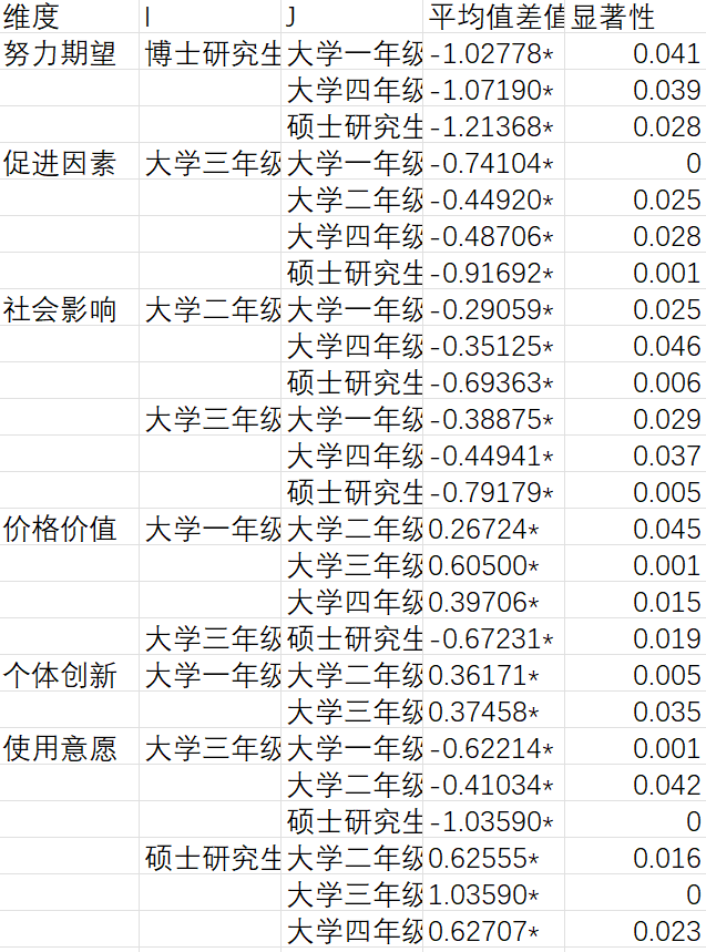
Further analysis was conducted for the significant variables. The specific results are shown in the following table (post hoc test — LSD):
| Dimension | I | J | Mean Difference (I-J) | Significance |
|---|---|---|---|---|
| Effort expectancy | Doctoral student | Freshman | -1.02778* | 0.041 |
| Senior | -1.07190* | 0.039 | ||
| Master’s student | -1.21368* | 0.028 | ||
| Facilitating conditions | Junior | Freshman | -0.74104* | 0 |
| Sophomore | -0.44920* | 0.025 | ||
| Senior | -0.48706* | 0.028 | ||
| Master’s student | -0.91692* | 0.001 | ||
| Social influence | Sophomore | Freshman | -0.29059* | 0.025 |
| Senior | -0.35125* | 0.046 | ||
| Master’s student | -0.69363* | 0.006 | ||
| Junior | Freshman | -0.38875* | 0.029 | |
| Senior | -0.44941* | 0.037 | ||
| Master’s student | -0.79179* | 0.005 | ||
| Price value | Freshman | Sophomore | 0.26724* | 0.045 |
| Junior | 0.60500* | 0.001 | ||
| Senior | 0.39706* | 0.015 | ||
| Junior | Master’s student | -0.67231* | 0.019 | |
| Personal innovativeness | Freshman | Sophomore | 0.36171* | 0.005 |
| Junior | 0.37458* | 0.035 | ||
| Behavioral intention | Junior | Freshman | -0.62214* | 0.001 |
| Sophomore | -0.41034* | 0.042 | ||
| Master’s student | -1.03590* | 0 | ||
| Master’s student | Sophomore | 0.62555* | 0.016 | |
| Junior | 1.03590* | 0 | ||
| Senior | 0.62707* | 0.023 |
Effort expectancy: doctoral students differ significantly from other grades or stages, including freshmen, seniors, and master’s students.
Facilitating conditions: juniors differ significantly from other grades or stages, including freshmen, sophomores, seniors, and master’s students. The difference from master’s students is especially significant (P = 0.001).
Social influence: the difference between sophomores and freshmen is significant, with P = 0.025. Juniors also differ significantly from freshmen, seniors, and master’s students, indicating significant grade-level differences in students’ perception of social influence.
Price value: freshmen differ significantly from sophomores, juniors, and seniors, and juniors also differ significantly from master’s students. This indicates that grade significantly affects students’ evaluation of price value.
Personal innovativeness: freshmen differ significantly from sophomores and juniors, indicating that students’ innovativeness varies across grades.
Behavioral intention: juniors differ significantly from freshmen, sophomores, and master’s students. The difference between master’s students and juniors is especially large, indicating that master’s students score much higher than undergraduates on behavioral intention.