
Operation Steps#
- Choose the analysis method: click “Analyze” in the menu bar, then choose “Descriptive Statistics,” and then click “Explore.”
- Set variables: add the variables to be tested into the “Dependent List” box.
- Choose plots: click the “Plots” button, select “Histogram” and “Normality plots with tests,” then click “Continue.”
- Run the analysis: click “OK” to start the analysis process.
Result Interpretation#
Inspect the Plots#
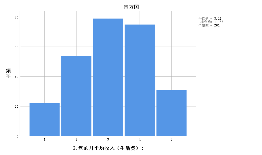
- Histogram: judge whether the data distribution is close to a normal distribution by observing the histogram. A normal distribution usually appears as a bell-shaped curve that is higher in the middle and lower at both ends.
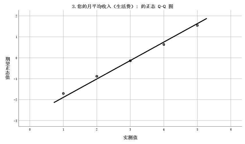
- Q-Q plot: check the distribution of data points in the Q-Q plot and confirm whether they align along the diagonal line. If the points are close to the diagonal line, the data distribution is close to normal.
Inspect the Table#
Looking at plots is only a convenient method; the more rigorous approach is to read the table. Scroll down and you will see a table named “Tests of Normality.” Mainly look at the significance value. If it is greater than 0.05, the data meet the normal-distribution assumption; if it is less than 0.05, the data do not meet the normal-distribution assumption. The table usually includes two test methods: the Kolmogorov-Smirnov test, abbreviated as the K-S test, and the Shapiro-Wilk test, abbreviated as the S-W test. They differ in applicability: the K-S test applies when the sample size is greater than 50; the S-W test applies when the sample size is less than 50.