
Video#
Click this text to watch the video version of this article
For more SPSS videos, see: SPSS video collection
Descriptive Statistics — Frequencies#
Terminology#
- Percentage: the frequency of a category or value divided by the total sample size (including missing values), multiplied by 100.
- Valid percentage: the frequency of a category or value divided by the valid sample size (excluding missing values), multiplied by 100.
- Cumulative percentage: percentages (or valid percentages) accumulated category by category from the first category onward, showing the cumulative distribution of the data.
- Other terms:
- Mean (M): the total sum of the data divided by the sample size; it reflects central tendency and is sensitive to extreme values.
- Median (D): the middle value after the data are ordered; suitable for skewed distributions or data with extreme values.
- Mode (Q): the value that occurs most often in the data; it may not be unique.
- Sum (S): the total of all numeric values.
- Standard deviation (I): measures data dispersion; a larger value means the data are more spread out.
- Minimum (I): the smallest value in the dataset, used to identify outliers or the data range.
- Maximum (×): the largest value in the dataset; together with the minimum, it defines the data range.
- Variance (V): the square of the standard deviation; it reflects the average degree to which data deviate from the mean.
- Range (N): the difference between the maximum and minimum values, showing the span of the data.
- Standard error of the mean (E): the fluctuation of the sample mean, used to estimate the confidence interval of the population mean.
Procedure#
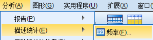
- Analyze → Descriptive Statistics → Frequencies
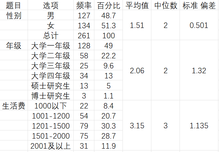
- Paste the table into Excel and format it as follows:
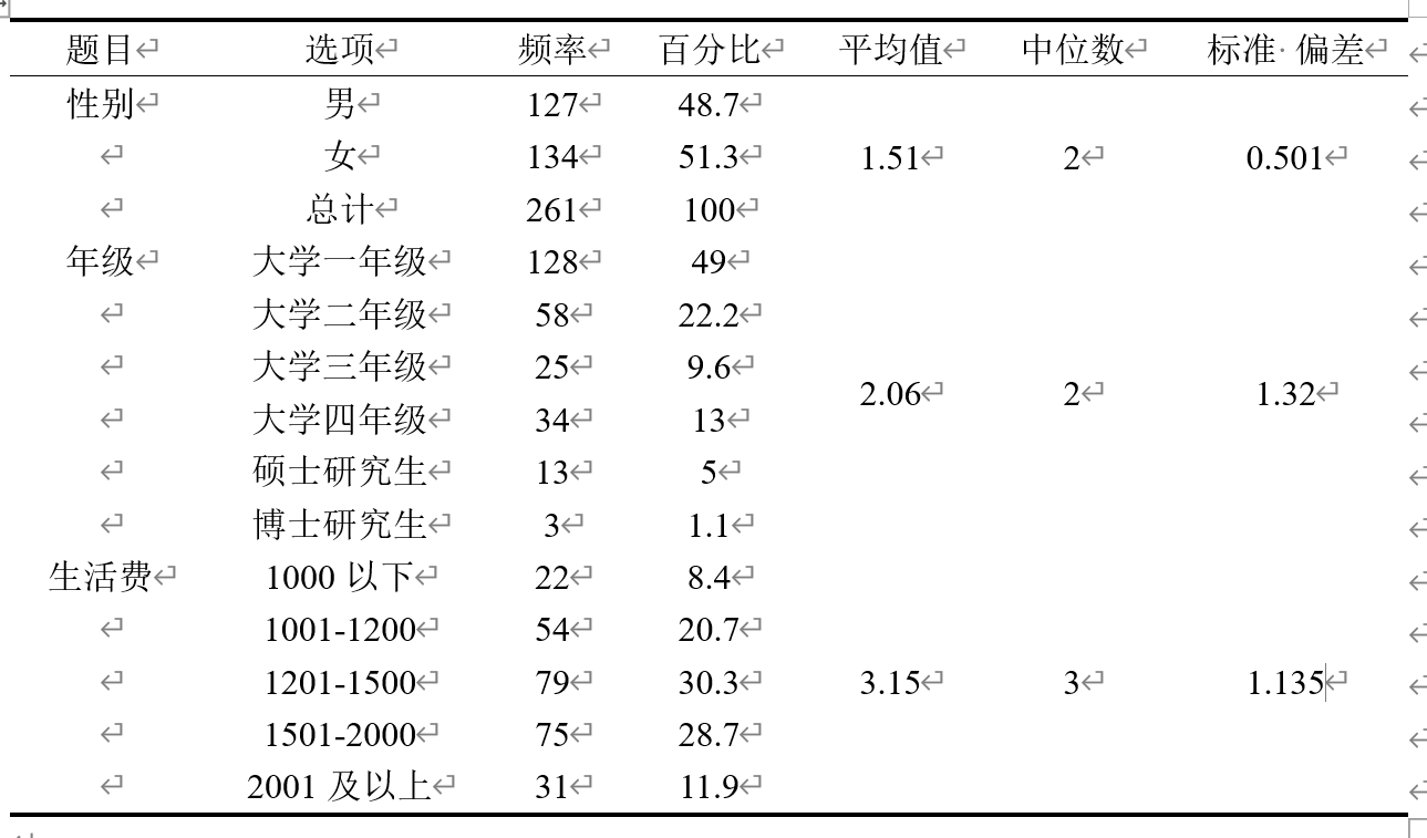
- Copy it into Word, turn it into a three-line table, and then explain it.
Descriptive Statistics — Crosstabs#
Preliminary Concepts#
- Suppose you want to analyze the relationship between “gender” and “smoking habits.” In a crosstab:
- “Gender” is placed in the column position.
- “Smoking habits” is placed in the row position.
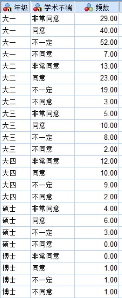
- Case weighting: if one row represents one case (person), weighting is not needed; if one row represents a category, weighting is needed.
Terminology#
Exact (X)#
- Asymptotic only (A):
- Definition: a class of statistical test methods based on large-sample theory. It assumes that when the sample size is large enough, the statistic’s distribution approaches a known distribution, such as a normal distribution. This method is especially effective for large samples, but it may be inaccurate for small samples.
- Application: for example, chi-square tests and t tests are usually based on asymptotic theory. Asymptotic methods obtain approximate results as the sample size gradually increases.
- Monte Carlo method (M):
- Definition: a statistical method that uses random simulation for approximate calculation. It uses many random samples to estimate probability distributions, calculate expected values, evaluate test significance, and so on. It is very suitable for complex problems that are difficult to solve with traditional analytical methods.
- Application: for example, simulating sample data to estimate the distribution of a test statistic and then calculating the p-value or significance level.
- Confidence level (C):
- Definition: in repeated experiments, the proportion of constructed confidence intervals that contain the unknown parameter. A 99% confidence level means there is a 99% probability that the interval contains the true parameter value, and a 1% probability that it does not.
- Application: for example, if you obtain a 99% confidence interval in an experiment, you can be 99% confident that the interval contains the population parameter.
- Number of samples (N):
- Definition: the number of individuals selected in a statistical experiment or survey. In hypothesis testing or simulation, sample size directly affects the accuracy and stability of the results.
- Application: the larger the sample size, the higher the test power usually is, and the better it can reflect population characteristics.
- Fisher’s exact test (E)
- Definition: exactness usually refers to how close an estimate is to the true value in a specific test. In statistical testing, precision is usually related to standard error; the smaller the standard error, the more precise the estimate.
- Application: high-precision statistical tests can produce more accurate conclusions and reduce error.
- Time limit for each test (T):
- Definition: the maximum allowed execution time for each test or simulation. In complex calculations or simulations, a time limit may be set for each test to save computing resources or improve efficiency in practical applications.
- Application: for large datasets or complex models, setting a time limit may be necessary to avoid excessive calculation time and program stagnation.
- Used when the sample is small or expected frequencies are low.
Statistics (S)#
Chi-square test (H)
- Definition: a commonly used test for assessing whether two categorical variables have statistically significant independence or association. It compares observed frequencies with expected frequencies.
- Application: commonly used in contingency-table analysis, such as testing whether gender is associated with a certain behavior.
Correlation (R)
- Definition: correlation measures the strength and direction of the linear relationship between two variables. Its value ranges from -1 to 1: -1 indicates a perfect negative correlation, 1 indicates a perfect positive correlation, and 0 indicates no relationship.
- Application: suitable for analyzing relationships between continuous variables.
Nominal
- Contingency coefficient (Q)
- Used to measure the strength of the relationship between two categorical variables. It is based on the chi-square test result and calculated by standardizing the chi-square statistic, representing the degree of association between categorical variables. Its value ranges from 0 to 1: 0 means no association, and 1 means complete association.
- Phi and Cramér’s V
- Phi coefficient (Φ):
- Definition: the Phi coefficient measures the association between two binary categorical variables in a 2×2 contingency table. Its value ranges from -1 to 1. 1: perfect positive association, meaning the ordering is completely consistent. -1: perfect negative association, meaning the ordering is completely opposite. 0: no association, meaning the ordering is completely independent.
- Use case: usually used for binary classification (2×2 contingency tables), such as the relationship between gender and smoking status.
- Cramér’s V coefficient:
- Definition: Cramér’s V is a standardized chi-square statistic suitable for contingency tables of any size, not only 2×2 tables. Its value is also between 0 and 1, where 0 means no association and 1 means complete association. Cramér’s V provides a standardized way to measure association strength, especially when the contingency table dimensions are greater than 2.
- Use case: suitable for relationship analysis between multi-category variables, especially when there are multiple categories; it is more commonly used than the Phi coefficient.
- Use in SPSS: when Phi and Cramér’s V are selected, SPSS calculates both statistics and provides association-strength measures according to your data size.
- Lambda
- Definition: Lambda is a measure of association strength between two categorical variables, especially suitable for categorical variables (nominal variables) and a dependent variable (or independent variable). Lambda ranges from 0 to 1; the larger the value, the stronger the association. Lambda mainly measures the relationship by calculating how much uncertainty in the dependent variable is reduced when the independent variable is known.
- Use case: when you need to measure the effect strength of one categorical independent variable on another categorical dependent variable, Lambda can be selected. For example, judging the effect of education level (independent variable) on occupation type (dependent variable).
- Use in SPSS: after Lambda is selected in crosstab analysis, SPSS calculates the value and provides information about the relationship strength between the independent and dependent variables.
- Uncertainty coefficient (U)
- Definition: the uncertainty coefficient measures dependency between two categorical variables and comes from information theory. It indicates how much uncertainty in one variable can be reduced when the value of another variable is known. Similar to Lambda, it reflects dependency between variables, but its calculation is based on information reduction. The uncertainty coefficient usually ranges from 0 to 1; the larger the value, the stronger the dependency.
- Use case: suitable for measuring complex dependencies between categorical data, especially useful in information asymmetry or uncertainty analysis.
- Use in SPSS: after selecting the uncertainty coefficient in crosstab analysis, SPSS calculates and displays the value to help you measure dependency between two categorical variables.
- Contingency coefficient (Q)
Ordinal
- Gamma
- Definition: Gamma measures the strength of the relationship between two ordinal categorical variables. It is especially suitable for analyzing ordinal data such as rating scales. Gamma measures ranking consistency between variable pairs, that is, whether the direction of one variable’s values is consistent with the ordering direction of the other variable’s values. Its value ranges from -1 to 1.
- Application: Gamma is often used for correlation analysis of ordinal categorical data, such as the relationship between education level and salary level, or associations between ordered survey response options such as “very satisfied,” “satisfied,” “neutral,” and “dissatisfied.”
- Use in SPSS: after Gamma is selected, SPSS calculates the Gamma value to measure consistency or association between two ordinal categorical variables.
- Somers’ d (S)
- Definition: Somers’ d is an asymmetric measure of relationship strength between two ordinal variables. It is especially suitable when one variable is treated as the dependent variable and the other as the independent variable. It is similar to Gamma but asymmetric, meaning it considers the directional dependency between independent and dependent variables. Somers’ d measures the effect strength of the independent variable on the dependent variable and ranges from -1 to 1.
- Application: Somers’ d is often used in ordinal data analysis to test the effect of an independent variable on a dependent variable, especially when directional influence must be considered, such as analyzing the effect of education level on income level.
- Use in SPSS: when Somers’ d is selected, SPSS calculates the statistic to help you understand how one ordinal variable affects changes in another ordinal variable.
- Kendall’s tau-b
- Definition: Kendall’s tau-b measures correlation between two ordinal variables. It is suitable for ordinal categorical data, especially when ties exist in the data. It measures correlation by calculating the ratio between concordant pairs and discordant pairs. Tau-b adjusts for ties and is suitable for larger contingency tables.
- Application: tau-b is suitable for ordinal data analysis, such as rating-scale data in questionnaires, and can handle ties, for example when two items receive the same rating.
- Use in SPSS: after Kendall’s tau-b is selected in SPSS, SPSS calculates the tau-b value and provides detailed information about the correlation strength between two ordinal variables.
- Kendall’s tau-c
- Definition: Kendall’s tau-c is another statistic for measuring correlation between ordinal variables. It is similar to tau-b, but it is used for larger contingency tables, especially when the number of rows and columns is unequal. Tau-c is also based on concordant and discordant pairs, and is more suitable for large tables. Its value also ranges from -1 to 1, indicating ranking consistency between two variables.
- Application: tau-c is especially suitable when the dimensions of the contingency table are large, such as analyzing associations among multiple ordered survey options.
- Use in SPSS: after Kendall’s tau-c is selected in SPSS, SPSS calculates the tau-c value and provides a measure of ordinal-data correlation in larger contingency tables.
- Gamma
Interval by interval
- Eta:
- Definition: used to evaluate the relationship between a categorical variable, such as gender, education level, or treatment group, and a continuous variable, such as income, score, or time. In crosstab analysis, if Eta is selected, SPSS calculates and reports the extent to which the categorical variable affects the continuous variable. This helps researchers understand the size of the independent variable’s effect.
- Eta:
Kappa
- Definition: the Kappa coefficient measures agreement between two observers or two measurement tools while excluding the effect of chance. It measures agreement beyond chance and is often used to test consistency in categorical data.
Risk (I)
- Used to measure the probability that an event occurs; often used in epidemiological analysis.
McNemar (M)
- Definition: the Cochran and Mantel-Haenszel test is used to analyze the relationship between two categorical variables while controlling for other possible confounding variables. By adjusting for control variables, the test helps examine independence or association between two categorical variables.
- Application: commonly used in epidemiological research to evaluate whether exposure and disease remain significantly associated after controlling for factors such as age and gender. For example, testing the relationship between smoking and lung cancer after controlling for age and gender.
Cochran and Mantel-Haenszel statistics (A)
- Test common odds ratio equals (T): when “test common odds ratio equals 1” is selected in crosstab analysis, SPSS performs a hypothesis test to determine whether the odds ratio equals 1, helping judge whether the relationship between two variables is significant.
Cells (E)#
- Counts (T):
- Observed (O): select the actual count data for analysis.
- Expected (E): select expected values for analysis, usually the expected frequency values used in chi-square tests.
- Hide small counts (H): hide counts smaller than a specified value during count calculation.
- Less than 5: means hiding observed counts smaller than 5, often used in frequency-table analysis to avoid very small frequencies affecting results.
- Z tests:
- Compare column proportions (P): compare column proportions, commonly used to test whether two proportions differ significantly.
- Adjust p-values (Bonferroni method): a multiple-comparison correction method mainly used to reduce the false rejection rate caused by multiple hypothesis tests.
- Percentages:
- Row (R): calculate row percentages, usually used in crosstab analysis.
- Column (C): calculate column percentages, also used in crosstab analysis.
- Total (T): calculate percentages for the entire dataset.
- Residuals:
- Unstandardized (U): residuals without standardization.
- Standardized (S): standardized residuals, making the residual scale uniform.
- Adjusted standardized (A): standardized residuals calculated after adjustment by a certain method, often used for multiple comparisons.
- Noninteger weights:
- Round cell counts (N): round cell counts.
- Round case weights (W): round case weights.
- Truncate cell counts (L): truncate cell counts without rounding.
- Truncate case weights (W): truncate case weights.
Steps#
- Select Crosstabs
- In the SPSS menu, choose “Analyze” → “Descriptive Statistics” → “Crosstabs.”
- Select variables
- In the Crosstabs dialog box, select the two variables you want to analyze:
- Drag one variable into the “Rows” box.
- Drag the other variable into the “Columns” box.
- Test of independence
- Click the “Statistics” (S) button and select “Chi-square” (H) in the dialog box:
- Run the test of independence to check whether the two variables are independent. SPSS uses the chi-square test to judge whether there is a statistically significant relationship between the row and column variables.
- Click the “Statistics” (S) button and select “Chi-square” (H) in the dialog box:
- Choose cell display
- Click the “Cells” button and choose the information you want displayed in the crosstab:
- Select “Observed Count” to show the actual observed frequency in each cell.
- Select “Expected Count” to show the expected frequency in each cell if the variables were not associated.
- You can also select “Column percentage,” “Row percentage,” or “Total percentage” to display different percentage data.
- Click the “Cells” button and choose the information you want displayed in the crosstab:
- Run the test
- After setting all options, click “OK”. SPSS calculates the crosstab and outputs the result.
- View the output
- SPSS generates a crosstab and provides the following output in the Chi-square test results:
- Chi-square statistic: chi-square value (H), degrees of freedom (df), and p-value.
- If the p-value is less than the significance level, such as 0.05, reject the null hypothesis and conclude that there is a significant association between the two variables. Conversely, if the p-value is greater than the significance level, accept the null hypothesis and conclude that the two variables are independent.
- Interpret the results
- Chi-square value: reflects the difference between observed and expected frequencies. The larger the value, the more significant the difference.
- Degrees of freedom: = (number of rows - 1) × (number of columns - 1)
- p-value:
- p < 0.05: reject the null hypothesis and conclude that the variables have a significant relationship.
- p >= 0.05: accept the null hypothesis and conclude that the variables do not have a significant relationship.
Multiple Response — Multiple-Choice Question Analysis#
Terminology#
Percentage and Percent of Cases#
Percentage:
$$ \text{Percentage} = \frac{\text{Number of cases}}{\text{Total number of all selected responses}} \times 100% $$
Percent of cases:
$$ \text{Percent of cases} = \frac{\text{Number of cases}}{\text{Total sample size}} \times 100% $$
Cell Percentages#
- Row (W): calculate percentages based on the total of the row variable. Use case: analyze how different row groups are distributed across the column variable.
- Column (C): calculate percentages based on the total of the column variable. Use case: analyze the share of different column options within the row variable.
- Total (T): calculate percentages based on the total sample size or total responses. Use case: view each cell’s share from an overall perspective.
- Match variables across response sets (M): when analyzing two multiple-choice questions, force SPSS to calculate the crosstab using the same set of samples, that is, complete pairing.
- Use case: ensure the samples for two multiple-choice questions are exactly the same, avoiding sample-size fluctuation caused by missing values.
- Example: when analyzing the relationship between “purchase channels” and “return reasons,” keep only samples that answered both questions.
Percentages Based On#
- Cases (S): the denominator is the total sample size, meaning each respondent is counted as 1. Use case: focus on “population proportion,” such as how many people selected both A and B.
- Responses (R): the denominator is the total number of responses, meaning each respondent’s multiple-choice answers are counted separately. Use case: focus on “answer proportion,” such as the share of A and B among all answers. Example: If 100 people each select an average of 2 purchase channels, the total responses equal 200:
- Based on cases: proportion of a selected channel = number of people who selected it / 100
- Based on responses: proportion of a selected channel = number of selections / 200
Missing Values#
- Exclude cases columnwise within dichotomies (E): if a respondent has a missing value in a multiple-choice question, such as not answering one option, exclude that respondent from the entire analysis. Impact: the sample size decreases, but all analyses are based on complete data.
- Exclude cases columnwise within categories (X): exclude cases only when the current classification variable, such as gender, has missing values; missing values in the multiple-choice question do not affect the analysis. Impact: retains relatively more samples.
Steps#
Set multiple-response variables
- Choose Analyze > Multiple Response > Define Variable Sets.
- In the dialog box:
- Select response variables: in the variable list, select all variables related to the multiple-choice question. For example, select “apple,” “banana,” and “orange.”
- Click the arrow to add these variables to the response variables box.
- Choose an encoding method:
- Dichotomies (D), with counted value (0): 1. A value of 1 means selected, and 0 means not selected. This is the most common method.
- Set a set name for the response variables, such as “favorite fruits.”
- Click Add, then click Continue.
Run frequency analysis
- After setting the multiple-response set, you can analyze the selection frequency of each option.
- Choose Analyze > Multiple Response > Frequencies.
Run crosstab analysis
- Choose Analyze > Multiple Response > Crosstabs.
- File > New > Data
- Copy the crosstab result, edit it in Excel into the following format, and choose “Paste with variable names (A)”:
- Data > Weight Cases > Weight cases by (W) > Frequency variable (E): frequency
- Choose Analyze > Descriptive Statistics > Crosstabs.
- Row variable: select the variable you want to analyze with the multiple-response set, such as gender.
- Column variable: select the multiple-response set, such as “favorite fruits.”
- Click Statistics and select Chi-square or another relevant statistic.
- Click Cells and choose whether to display Observed Count, Expected Count, and Percentages.
- Choose Analyze > Multiple Response > Crosstabs.